I’m in the middle of a long-term project—I’m building a Senate election model and writing about the process as I go (see previous posts here). At this point I’ve written a lot of the code and I was tempted to devote this update to how I’m aggregating polls, forecasting final vote shares, or thinking about error. But before writing any of those more technical posts, I want to devote some space to a time-honored mathematical tradition: the sanity check.
The sanity check isn’t a specific algorithm or theorem or anything like that—it’s more of an intuitive process that helps you keep your eye on the prize when you’re trying to figure something out.
If you’ve been working on a tough math problem for a while, it’s easy to lose track of reality—to get submerged in the world of math, try out a bunch of creative (and sometimes questionable) techniques to solve your problem, and then feel disoriented when you finally emerge and look at the results. At that point, it’s a good idea to take a step back, think about what your answers should look like, maybe run a few short tests, and make sure that your results don’t seem totally bananas.
If you get a weird result, you should head back into the data and code and check your work. Your oddball predictions really might be a new, exciting discovery! But it’s more likely the result of a bad assumption or a bug in your code.
I decided to set up the raw materials for two sanity checks early in the process. First, I wanted a sense of how accurate a very basic poll average is at any given point in time. If my model is less accurate than this baseline, then I’m doing something wrong. Second, I wanted a ballpark of how various polling leads translate into win probabilities. If my model outputs look bad in light of these estimates, that’s a potential warning sign. Now obviously there are more sophisticated tests and standards (calibration seems to be the right measure for probabilistic models), but this is the sanity check. It’s only supposed to help you keep your bearings when you’re deep in the data.
I started out by keeping it simple and looking into how often the leader in a straightforward poll average ended up winning the race every day from Election Day to 200 days prior. For every race in my dataset (which in this case is a combination of publicly available polls from the New York Times, RealClearPolitics and the Huffington Post), I calculated the average margin in the previous three polls of the race (in races that had only one or two polls, I just averaged what I had). There were no fundamentals, no accounting for past accuracy, sample size, partisanship or anything—just a simple average. I then calculated the percentage of races (with polling) where the poll leader won the race.
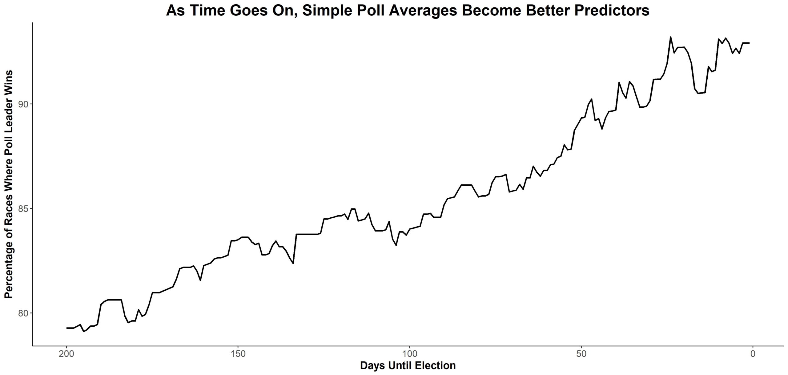
This is a really encouraging graphic. Basically it says that even at this point in the cycle (a little less than 200 days out) our poll averages tell us something about which candidates will win and lose. And when we’re close to Election Day, a simple average will correctly project the winner a little over 90 percent of the time. A 92 percent to 93 percent hit rate is far from perfect. If races were independent (and they’re not—sometimes polls in many races err in the same direction), a 92 percent to 93 percent error could easily map onto two or three missed calls. But this suggests that polls tell us something real and gives us a baseline for model accuracy on any day from now until Election Day.
This upward trend also highlights two important aspects of Senate races.
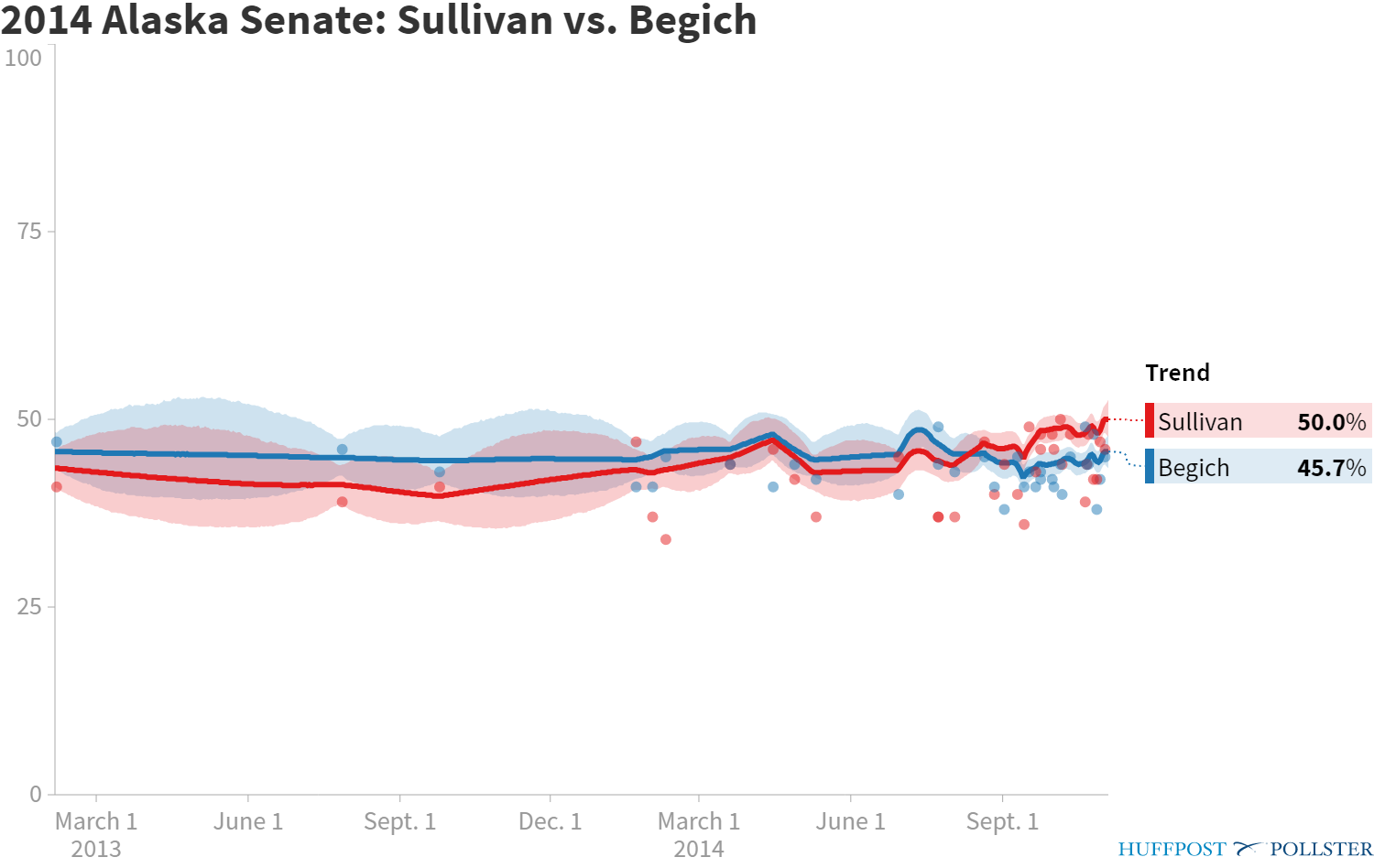
The first is that voters make up their mind as time goes on. For example, in 2014 Republican Dan Sullivan unseated Democratic Sen. Mark Begich in Alaska—but Begich was ahead for much of the race according to the Huffington Post’s Pollster aggregate.
These shifts can come very late in the cycle. In the 2016 Indiana Senate race, Democratic former Sen. Evan Bayh was tied with or ahead of Republican then-Rep. Todd Young in every poll listed on RealClearPolitics prior to November. But Young managed to barely get ahead in the average before Election Day and ended up winning the seat. That sort of late movement explains some of the overall trend towards accuracy.
The second involves which races are polled. You can think of the next graphic as exposing a bias in the first one, because sometimes pollsters wait until later in the cycle to poll less interesting (read: less competitive) races. And adding those easy-to-predict races should help lift that first line.
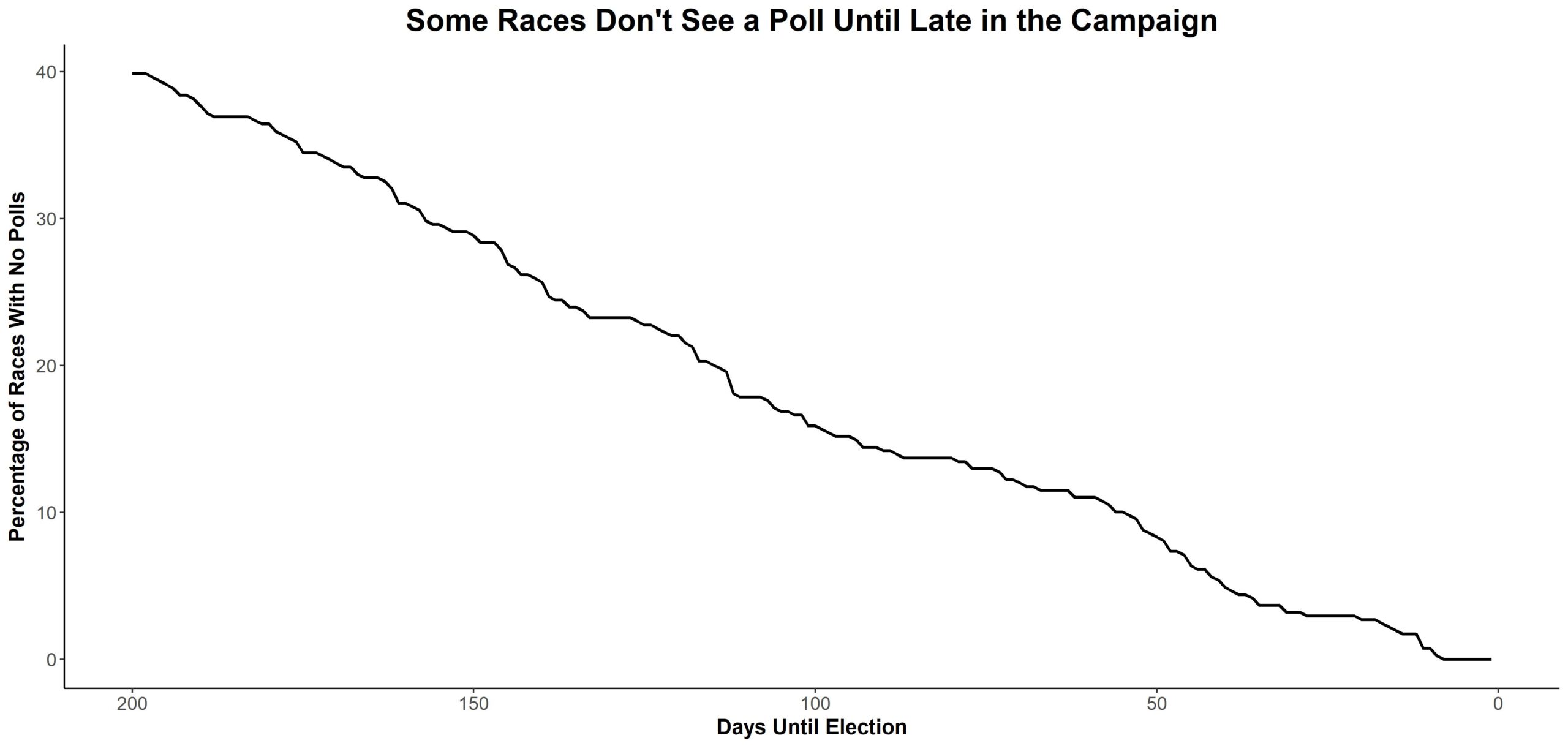
This graphic shows the percentage of races in our dataset that have no polls on a given day. The number starts out high (as one might expect, as not every race gets an early poll) and declines over time.
Some of these unpolled races aren’t competitive. For example, the dataset doesn’t have polls until the last month or two in the 2006 and 2008 Delaware Senate elections. But you didn’t need polling to do the math—both years featured a Democratic incumbent in a blue state during a blue wave. Similarly, there was no polling in the Iowa Senate race for roughly half of the time period shown in the graphic. But when data finally did show up, it (predictably) showed popular Republican incumbent Chuck Grassley winning by a landslide.
This logic applies to 2018 as well. I haven’t seen any polls of the Nebraska or Washington Senate election. But I’m a lot more sure about the outcome (Democrat Maria Cantwell and Republican Deb Fischer are strong favorites in Washington and Nebraska respectively) than I am about Florida or Arizona, where we already have a bit of polling.
The bird’s eye view here is that simple poll averages really can help us get some certainty in most Senate races. It also gives us an extremely rough baseline for how much accuracy might increase over time in a simplistic election model (the first graphic), while highlighting one of its blind spots (the third graphic).
These are helpful insights, but we can go deeper.
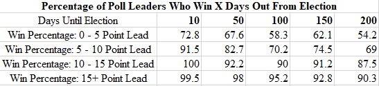
This table shows how often a poll average correctly picks a winner at various points in the election cycle. It’s not hard to read it—if you wanted to know how often a candidate who leads by zero to five points 200 days from the midterms (close to now) ended up winning their race, you’d look at the top right hand corner of the table. That number is 54 percent—indicating that a modest lead at this point in the cycle gives either candidate close to a coin toss chance of winning.
In that way, this table is a very basic model. It’s not a set of equations and it wouldn’t predict the Senate elections as well as the code I’ve written or the models at The Upshot or FiveThirtyEight. But it’s a way of thinking. It allows you to supply an input (the current polling average), think about the data in a principled way, and come up with a very rough win probability for a candidate at a given time.
I don’t advise using this table as a full-scale predictive model—it’s naïve about the polls, it doesn’t take correlated error (the idea that polls could fail in the same direction) into account, it groups races with a 0.4 point lead and a 4.0 point lead together, etc. Maybe most importantly, it suffers from the biases that the second graphic displays—that is, it’s looking at a smaller set of races when we’re 200 days than we are at 100, 50, or 10 days beforehand.
But it’s not supposed to be perfect. It’s a sanity check. The goal is to help you keep your bearings—to make sure that if you’re model (mental or otherwise) is spitting out an insane result, you know that and can adjust accordingly.